Show code
# Load necessary libraries for DA
library(MASS)
library(ggplot2)
library(caret)
library(ggfortify)Discriminant Analysis (DA) is a statistical technique used for classification and dimensionality reduction.
In simple terms, it’s used when we want to be able to decide whether an observation is ‘something’, or ‘something else’, based on what we know about it.
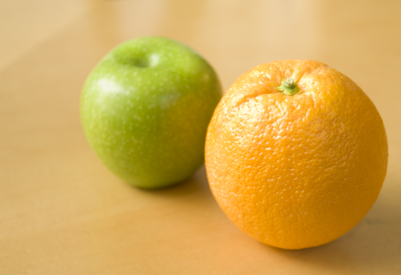
In the image below, you immediately recognise that one object is an apple, and one is an orange. DA tries to examine why you are able to tell the difference.
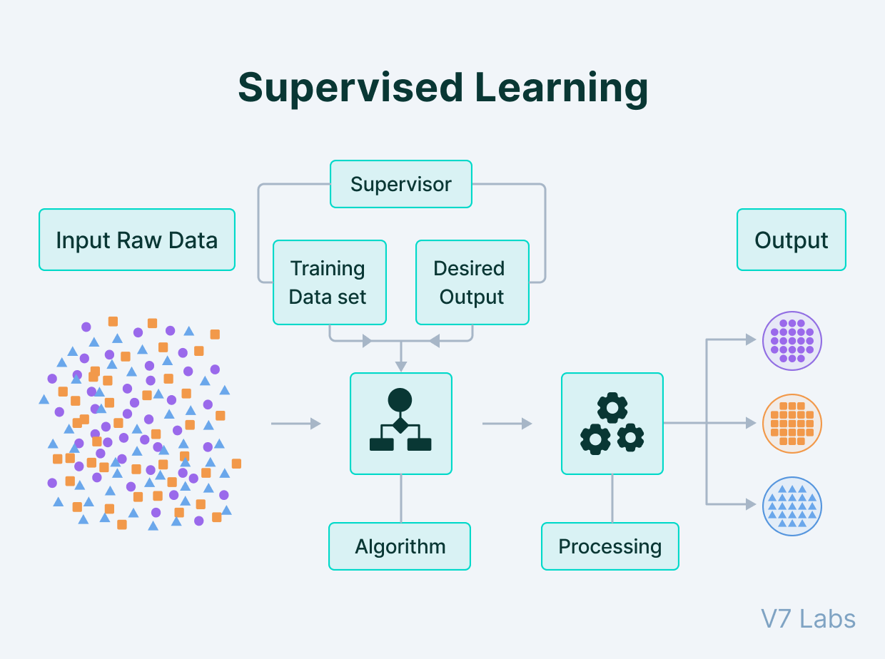
It’s particularly useful in the context of supervised learning (see below), where the goal is to assign observations to predefined classes based on several predictor variables.
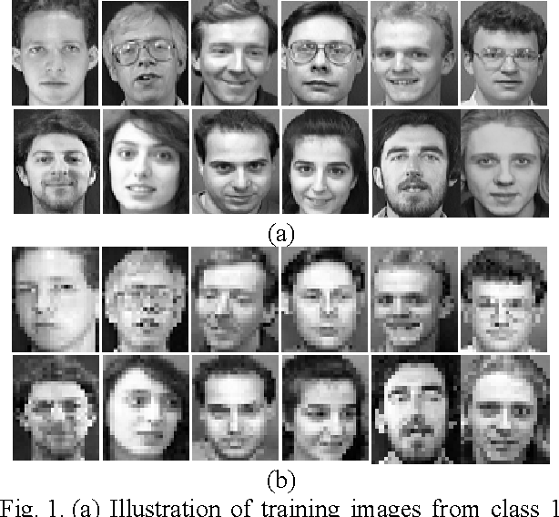
Imagine you’re developing a ‘fan recognition’ programme that will run at the turnstiles in your stadium. You might want to automate the process (for example) of detecting the age profile of each person coming into the stadium. You could use Discriminant Analysis to decide what features can be extracted from an image that would help you accurately classify a person’s age.
The term ‘supervised learning’ may be unfamiliar to you.
Imagine you’re teaching a child to recognise different types of fruits. You show them an apple and say, “This is an apple.” Then you show them a banana and tell them, “This is a banana.”
What you’re doing is giving them examples of different fruits and naming each one. You are assuming that the child will learn to recognise the features of an apple that lets them detect that it’s an apple, and the same with the banana.
This is similar to how supervised learning works in statistics and computer science. We assume that there are features of each object that make it different from others, and that recognising each type of object is based on detecting the presence (or absence) of these features.
In supervised learning, we give the software a set of examples, just like showing fruits to a child. But instead of fruits, the program gets data.
This data is special because it comes with answers. For example, a set of photos where each photo is labeled with the name of the object in it (like “dog,” “cat,” “car,” etc.). In the stadium example above, we might show the software pictures of thousands of supporters, and also tell it what age each supporter is.
Here’s what makes supervised learning interesting:
Learning with labels: Just like you labeled the fruits for the child, in supervised learning, the data the program gets is labeled. If it’s a picture of a dog, it comes with the label “dog.” If it’s a picture of someone who is 50 years old, it’s labeled with this information. This helps the program learn what each piece of data represents.
Two main jobs: Supervised learning can do two main things:
Classification: This is like sorting things into different groups. For example, sorting emails into “spam” and “not spam”, or “over 50” and “under 50”.
Regression: This is when the program predicts a number. For example, predicting the price of a house based on its size, location, etc.
Training: The process of learning from labeled data is often called “training.” The program looks at many examples and tries to understand the patterns. For instance, after seeing many photos of cats and dogs, it starts to recognise features that distinguish cats from dogs, or younger supporters vs. older supporters.
Testing: After the program has learned from the examples, it’s tested with new data it hasn’t seen before. This is to check how well it has learned.
Supervised learning is like teaching a computer to recognise or predict things by showing it examples, while giving it the correct answers.
On that basis, it can then go on to predict/recognise what new things are, because it already knows the features of the basic objects.
There are two main forms of Discriminant Analysis: Linear (LDA) and Quadratic (QDA).
LDA operates on a specific assumption: it assumes that these categories (or classes, as statisticians call them) each have data that follows a bell-shaped curve, technically known as a Gaussian distribution.
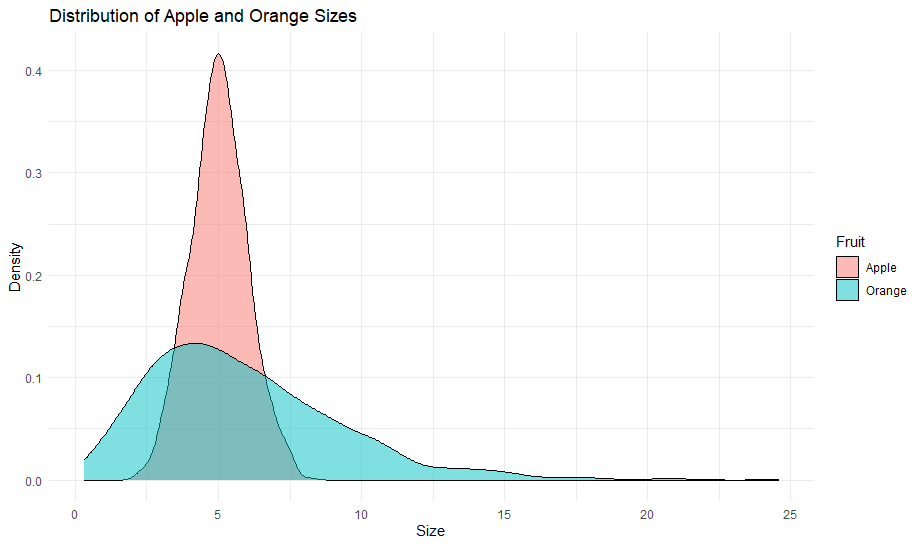
Picture this (we’ll stick to fruit for now!): if you were to plot the size of apples (your ‘class’), you’d get a bell curve where most apples are of average size, and a few are really small or really large.
Here’s the crucial bit: LDA assumes that while these bell curves for each fruit type have different centres (or means, in statistical terms), they spread out or vary in the same way. This spread or variation is captured by something called a covariance matrix, and LDA assumes that this matrix is the same for all fruit types.
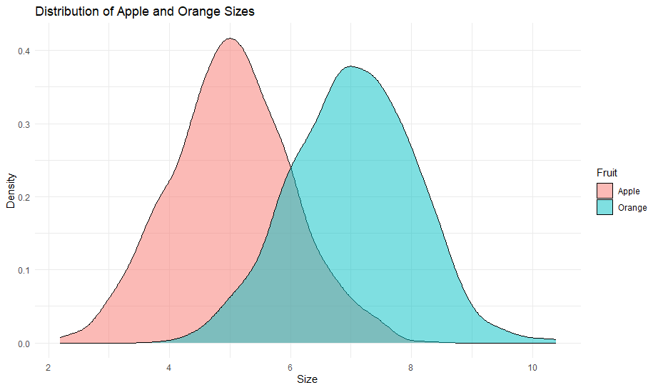
So, while apples might be, on average, smaller than oranges, the way their sizes vary around the average is assumed to be the same.
QDA is similar to LDA but with a key difference. QDA doesn’t make the same assumption about the covariance matrix being the same for all classes.
Going back to our fruit example, QDA would say, “Hold on, maybe the way apple sizes vary around their average is different from how orange sizes vary around their average.” In simpler terms, not only do the average sizes differ, but also the way they spread out from their average is different for each type of fruit.
This makes QDA a bit more flexible than LDA. It can adapt to more complex situations where each category (like each type of fruit) behaves quite differently not just in terms of its average, but also in how much variation there is around that average.
LDA is like saying, “Let’s assume our categories are different, but they vary in a similar way.” QDA, on the other hand, says, “Let’s not make that assumption; each category might vary in its own unique way.”
The assumptions of DA are similar to those that apply for the other procedures we have discussed in this module:
Multivariate normality: Data in each group should be approximately normally distributed.
Homoscedasticity: In LDA, the assumption is that all groups have the same covariance matrix. In QDA, this doesn’t apply.
Independence: Observations should be independent of each other.
Sample size: The sample size should be sufficiently large compared to the number of features.
To help understand Discriminant Analysis, I’ll show you an annotated example.
Don’t worry too much about the R code for now; we’ll cover that in more detail in the practical that follows.
# Load necessary libraries for DA
library(MASS)
library(ggplot2)
library(caret)
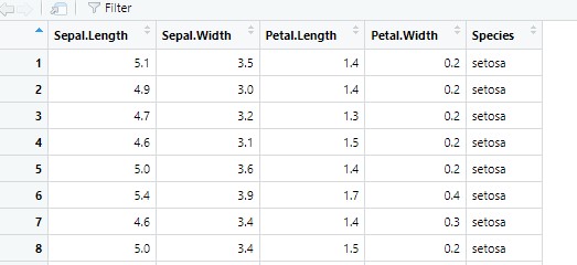
library(ggfortify)I’m going to use the iris dataset available in R, which is ideal for classification problems.
From the following screenshot, you can see that the dataset contains four variables with information about the features of the observation, and a fifth variable that names the species. So we know four things about the object, and it’s name.
# Load the iris dataset
data(iris)
set.seed(123)  # Setting seed for reproducibility

# Splitting the dataset into training and testing sets
index <- createDataPartition(iris$Species, p=0.7, list=FALSE)
train_data <- iris[index,]
test_data <- iris[-index,]The code above splits the data into two ‘sets’; training and testing. This is our first move into some concepts that will be crucial moving forward.
The main goal of splitting data is to assess the performance of a predictive model on unseen data. It helps in evaluating how well the model generalises beyond the data it was trained on.
Training Set:
This is usually the larger portion of our dataset, typically 70-80%.
The model learns from this data. It’s used to train the model and adjust its parameters.
Testing Set:
Usually smaller, often 20-30% of the dataset.
It’s kept separate and not used during the training phase.
After the model is trained, this set is used to evaluate its performance. It acts as new, unseen data for the model.
The first step is to create a model, trained on the ‘training data’.
We’ll create a LDA model.
Note that, at this point, we are telling the model what we know about the features associated with a particular category in our data (we will learn more about this code in this week’s practical):
# Fitting LDA model
lda_model <- lda(Species ~ ., data=train_data)

# Summary of the model
print(lda_model)
Call:
lda(Species ~ ., data = train_data)
Prior probabilities of groups:
setosa versicolor virginica
0.3333333 0.3333333 0.3333333
Group means:
Sepal.Length Sepal.Width Petal.Length Petal.Width
setosa 4.991429 3.365714 1.471429 0.2314286
versicolor 5.942857 2.777143 4.262857 1.3285714
virginica 6.631429 2.982857 5.591429 2.0342857
Coefficients of linear discriminants:
LD1 LD2
Sepal.Length 0.8603517 -0.02531284
Sepal.Width 1.3884435 -2.37490707
Petal.Length -2.2730220 0.89795664
Petal.Width -2.9135037 -2.68733735
Proportion of trace:
LD1 LD2
0.992 0.008 Now, we’re going to test how good our model is at identifying or predicting categories. We can do this because we have a subset of the data that hasn’t been used this, which gives us an opportunity to check our model’s accuracy at prediction.
# Predicting on test data
lda_pred <- predict(lda_model, test_data)
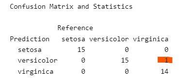
confusionMatrix(lda_pred$class, test_data$Species)Confusion Matrix and Statistics
Reference
Prediction setosa versicolor virginica
setosa 15 0 0
versicolor 0 15 1
virginica 0 0 14
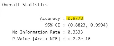
Overall Statistics
Accuracy : 0.9778
95% CI : (0.8823, 0.9994)
No Information Rate : 0.3333
P-Value [Acc > NIR] : < 2.2e-16
Kappa : 0.9667
Mcnemar's Test P-Value : NA
Statistics by Class:
Class: setosa Class: versicolor Class: virginica
Sensitivity 1.0000 1.0000 0.9333
Specificity 1.0000 0.9667 1.0000
Pos Pred Value 1.0000 0.9375 1.0000
Neg Pred Value 1.0000 1.0000 0.9677
Prevalence 0.3333 0.3333 0.3333
Detection Rate 0.3333 0.3333 0.3111
Detection Prevalence 0.3333 0.3556 0.3111
Balanced Accuracy 1.0000 0.9833 0.9667Don’t worry too much about the output for now. However, notice the ‘Accuracy’ statistic that is produced (0.98). This suggests that we’ve trained our model to be effective at identifying class (setosa, versicolor, virginica) based on the features we can observe about them.
In the ‘Confusion Matrix’ that precedes that statistic, you can see how often the model has failed to correctly identify the object (in this case, it made one error). This supports the idea that the model is effective at making predictions, based on what we tell it.
Here are some plots that help demonstrate the LDA process:
# Load libraries
library(MASS)  # For LDA

# Load the iris dataset
data(iris)

# Perform LDA
lda_model <- lda(Species ~ ., data = iris)

# Predict using the LDA model
lda_pred <- predict(lda_model)

# Add LDA components to the original data
iris_lda <- cbind(iris, lda_pred$x)

# Plot 1: LDA Components
ggplot(iris_lda, aes(LD1, LD2, color = Species)) +
  geom_point() +
  ggtitle("LDA: Iris Data") +
  xlab("Linear Discriminant 1") +
  ylab("Linear Discriminant 2")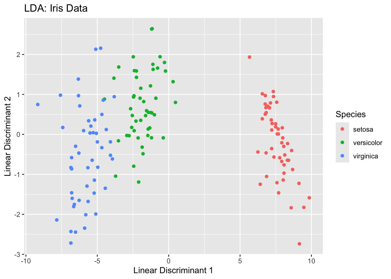
# Plot 2: LDA Components with Ellipses
ggplot(iris_lda, aes(LD1, LD2, color = Species)) +
  geom_point() +
  stat_ellipse(type = "norm") +
  ggtitle("LDA with Confidence Ellipses") +
  xlab("Linear Discriminant 1") +
  ylab("Linear Discriminant 2")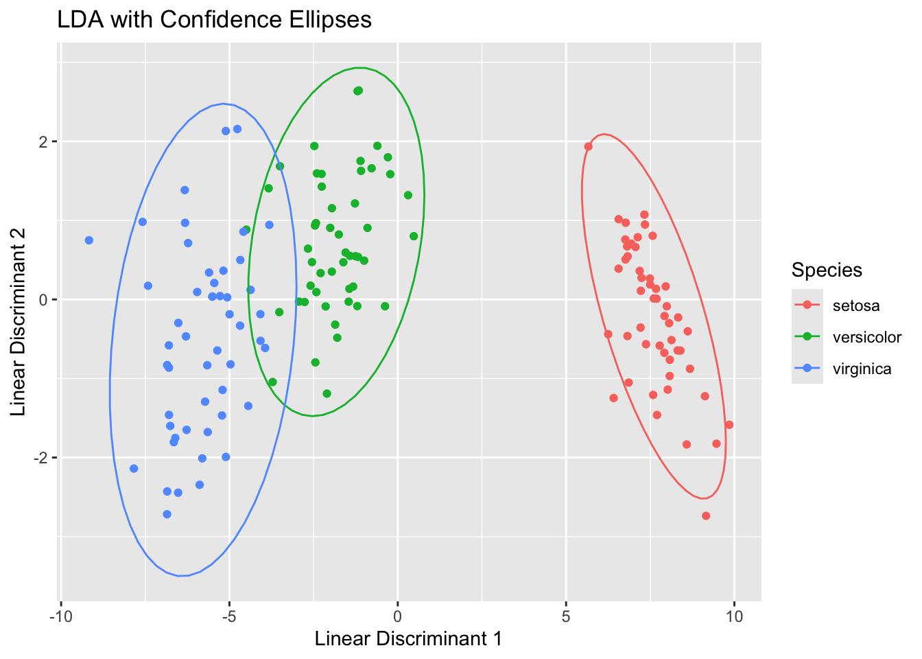
# Plot 4: LDA Component 1 by Species
ggplot(iris_lda, aes(Species, LD1, fill = Species)) +
  geom_boxplot() +
  ggtitle("Boxplot of LD1 by Species")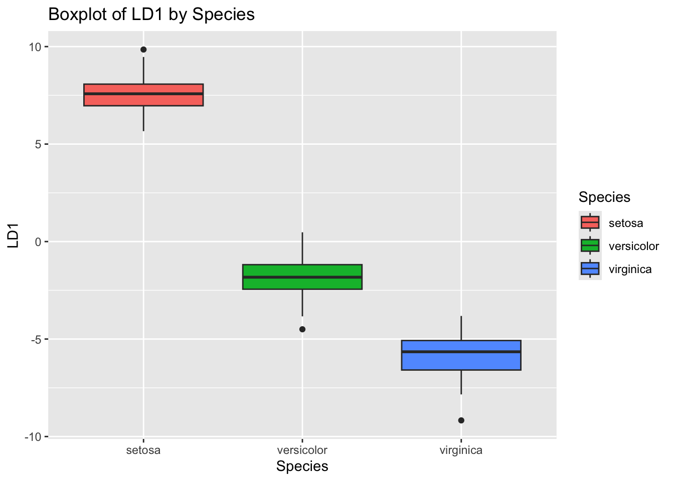
# Plot 5: LDA Component 2 by Species
ggplot(iris_lda, aes(Species, LD2, fill = Species)) +
  geom_boxplot() +
  ggtitle("Boxplot of LD2 by Species")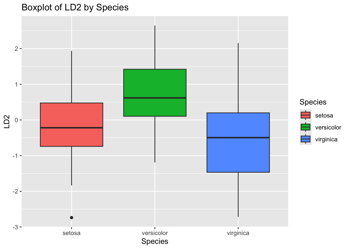
LDA is generally preferred when the sample size is small or when the predictors are highly correlated.
QDA may perform better when the class distributions are significantly different.
I wonder if you can think of some situations in sport data analytics where Discriminant Analysis could be useful?